Causal Impact

Causal Impact Analysis

What is it?

CausalImpact is an R package for causal inference using Bayesian structural time-series models. It implements an approach to estimate the causal effect of a designed intervention on a time series. For instance, in the following example, we calculate the impact that the VolksWagen Emissions Scandal had on their stock price.

The package was developed and open sourced by Google, for more information:

• Visit the project’s GitHub page
• Read the documentation and examples
• Read the research paper

How does it work:

Given a response time series (e.g., clicks) and a set of control time series (e.g., clicks in non-affected markets or clicks on other sites), the package constructs a Bayesian structural time-series model. This model is then used to try and predict the counterfactual, i.e., how the response metric would have evolved after the intervention if the intervention had never occurred.

There are two ways of running an analysis with the CausalImpact R package. You can either let the package construct a suitable model automatically or you can specify a custom model. In the former case, the kind of model constructed by the package depends on your input data:

• If your data contains no predictor time series (i.e., the data argument is a univariate time series), then the model contains a local level component and, if specified in model.args, a seasonal component. It’s generally not recommended to do this as the counterfactuals predicted by your model will be overly simplistic. They are not using any information from the post-period. Causal inference then becomes as hard as forecasting. Having said that, the model still provides you with prediction intervals, which you can use to assess whether the deviation of the time series in the post-period from its baseline is significant.
• If your data contains one or more predictor time series (i.e., the data argument has at least two columns), then, on top of the above, the model contains a regression component. In all practical cases I’ve seen it really is the predictor time series that make the model powerful as they allow you to compute much more plausible counterfactuals. I’d generally recommend adding at least a handful of predictor time series.

Underlying assumptions:

The main assumption is that there is a set control time series that were themselves not affected by the intervention. If they were, we might falsely under- or overestimate the true effect. Or we might falsely conclude that there was an effect even though in reality there wasn’t. The model also assumes that the relationship between covariates and treated time series, as established during the pre-period, remains stable throughout the post-period.

Data Collection

We will use the get.hist.quote() function of the tseries package to retrieve all the relevant stock prices, ggplot2 to create some of the charts and of course CausalImpact to perform the analysis. Let’s start by installing and loading all the necessary libraries:

options(warn = -1)
#install.packages("tseries")
library(tseries)
#install.packages("ggplot2")
library(ggplot2)
#devtools::install_github("google/CausalImpact")
library(CausalImpact)

We first extract the Adjusted Close price for all required stocks and I specifically chose the zoo format as it is the recommended object type to be used with CausalImpact. I’m including VolksWagen’s stock as well as BMW and Allianz Insurance; the last two will be used as regressors of the VW series in the second part of the analysis. The Emissions Scandal broke on Friday the 18th of September 2015, so I’m going to collect weekly data from the beginning of 2011 up to current date.

start = '2011-01-03'
  end = '2017-03-20'
quote = 'AdjClose'
VolksWagen <- get.hist.quote(instrument = "VOW.DE", start, end, quote, compression = "w")
BMW <- get.hist.quote(instrument = "BMW.DE", start, end, quote, compression = "w")
Allianz <- get.hist.quote(instrument = "ALV.DE", start, end, quote, compression = "w")
series <- cbind(VolksWagen, BMW, Allianz)

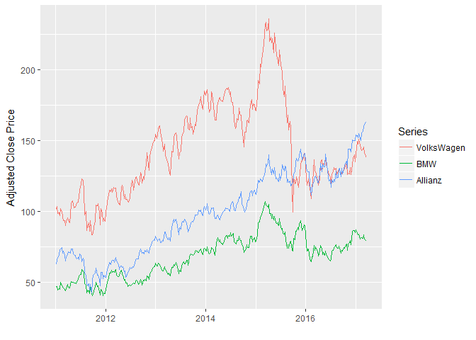
We then plot the three time series.

colnames(series) <- c("VolksWagen", "BMW", "Allianz")
autoplot(series, facet = NULL) + xlab("") + ylab("Adjusted Close Price")

We need to define the pre- and post-intervention periods (the emission scandal started on the 18th of September 2015)

pre.period <- as.Date(c(start, "2015-09-14"))
post.period <- as.Date(c("2015-09-21", end))

A Simple Model

The Causal Impact function needs at least three arguments: data, pre.period and post.period. The easiest way to perform a causal analysis is to provide only the series where the intervention took place as the data input and specify the seasonality frequency in the model.args parameter. This is equivalent as specifying a local level model with a seasonality component:

impact_vw <- CausalImpact(series[, 1], pre.period, post.period, model.args = list(niter = 1000, nseasons = 52))
plot(impact_vw)

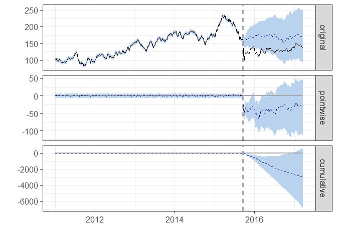
summary(impact_vw)

## Posterior inference {CausalImpact}
## 
##                          Average      Cumulative    
## Actual                   130          10252         
## Prediction (s.d.)        168 (24)     13285 (1901)  
## 95% CI                   [123, 217]   [9722, 17124] 
##                                                     
## Absolute effect (s.d.)   -38 (24)     -3033 (1901)  
## 95% CI                   [-87, 6.7]   [-6873, 529.7]
##                                                     
## Relative effect (s.d.)   -23% (14%)   -23% (14%)    
## 95% CI                   [-52%, 4%]   [-52%, 4%]    
## 
## Posterior tail-area probability p:   0.04928
## Posterior prob. of a causal effect:  95.072%
## 
## For more details, type: summary(impact, "report")

A quick look at the output should convince you that this method is probably not the best, at least for this data, as the confidence intervals of the estimates increases drastically with time.

Including Regressors

We can try to improve our model by supplying one or more covariates so that we’re basically performing a regression on our response variable. We will use the BMW and Allianz stock prices to explain our target series (you may argue that those series - especially BMW - may have been influenced by the scandal as well and that may be true, but certainly at a lower magnitude):

impact_vw_reg <- CausalImpact(series, pre.period, post.period, model.args = list(niter = 1000, nseasons = 52))
plot(impact_vw_reg)

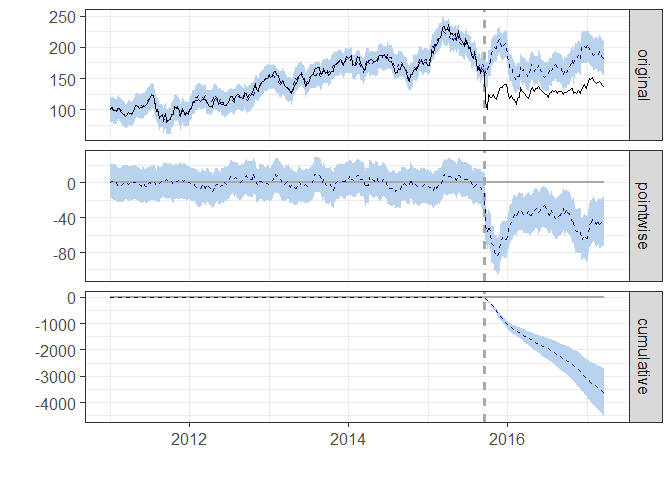
summary(impact_vw_reg)

## Posterior inference {CausalImpact}
## 
##                          Average        Cumulative    
## Actual                   130            10252         
## Prediction (s.d.)        176 (5.9)      13874 (463.3) 
## 95% CI                   [163, 187]     [12905, 14765]
##                                                       
## Absolute effect (s.d.)   -46 (5.9)      -3622 (463.3) 
## 95% CI                   [-57, -34]     [-4514, -2653]
##                                                       
## Relative effect (s.d.)   -26% (3.3%)    -26% (3.3%)   
## 95% CI                   [-33%, -19%]   [-33%, -19%]  
## 
## Posterior tail-area probability p:   0.001
## Posterior prob. of a causal effect:  99.8997%
## 
## For more details, type: summary(impact, "report")

The output of this second analysis looks much better: the confidence intervals of the estimate are fairly stable over time. Since we’re looking at stock prices, we shouldn’t look at the cumulative effect, but focus on the Average section.

The console output shows you the actual vs predicted effect (Average) as well as the absolute and relative effect. The output of the second analysis is saying that the Emissions Scandal brought down VolksWagen stocks by 26% - from a predicted $176 to an actual $130.

Another hint in favor of the latter model is given by the Standard Deviation of the estimates, which was 24 in the first model and is now down to 5.9.